


This post “Torchvision Semantic Segmentation,” is part of the series in which we will cover the following topics.
1. What is Semantic Segmentation?
Semantic Segmentation is an image analysis procedure in which we classify each pixel in the image into a class.
This is similar to what humans do all the time by default. Whenever we look at something, we try to “segment” what portions of the image into a predefined class/label/category, subconsciously.
Essentially, Semantic Segmentation is the technique through which we can achieve this with computers.3
You can read more about Segmentation in our post on Image Segmentation.
Let’s focus on the Semantic Segmentation process.
Let’s say we have the following image as input.

After semantic segmentation, you get the following output:

As you can see, each pixel in the image is classified to its respective class. For example, the person is one class, the bike is another and the third is the background.
This is, in most simple terms, what Semantic Segmentation is – identifying and separating each of the objects in an image and labeling them accordingly.

2. Applications of Semantic Segmentation
The most common use cases for Semantic Segmentation are:
2.1. Autonomous Driving
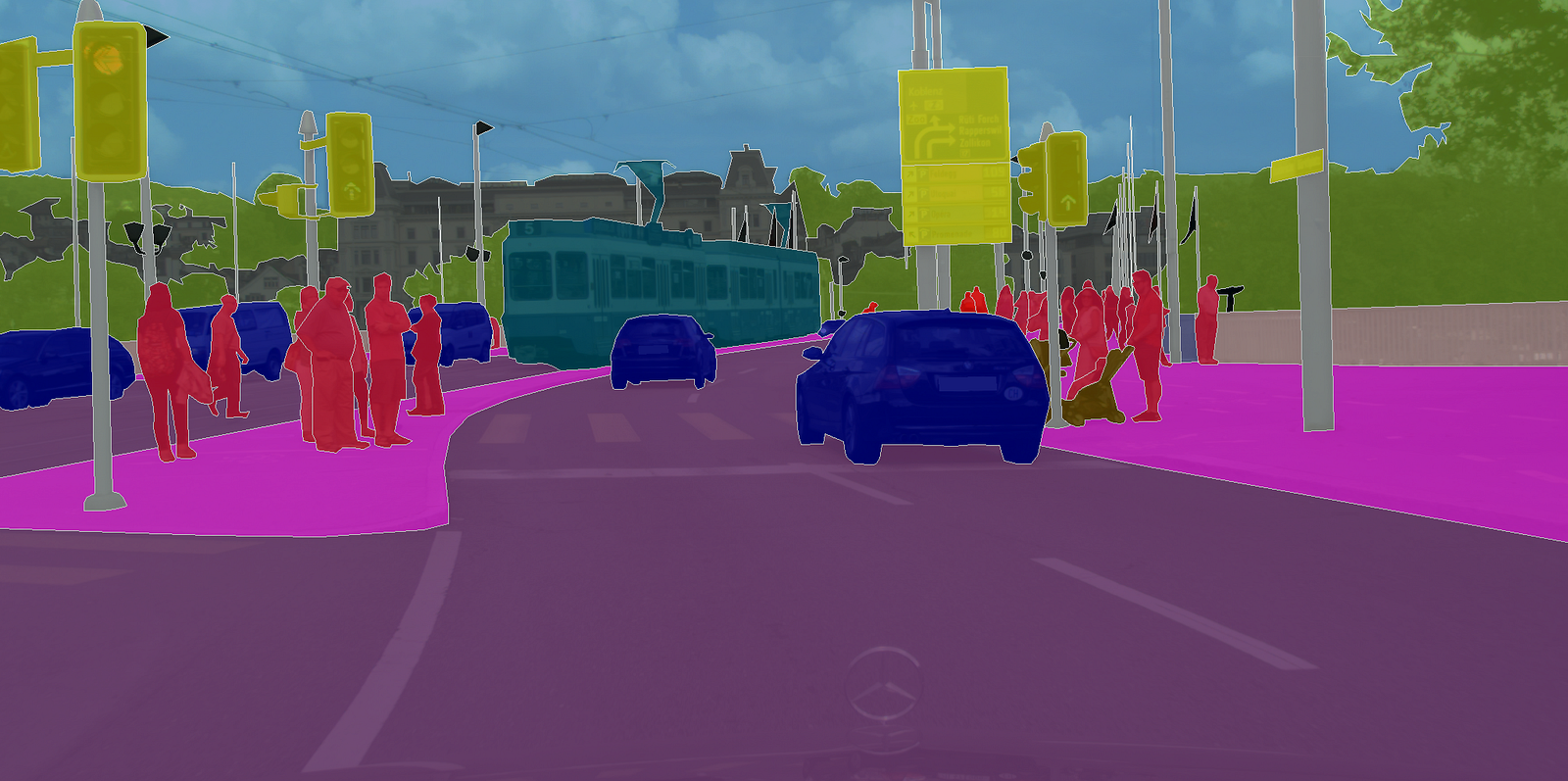
Source: CityScapes Dataset
In autonomous driving, the computer driving the car needs to have a good understanding of the road scene in front of it. It is important to segment out objects such as cars, pedestrians, lanes, and traffic signs. We cover this application in great detail in our Deep Learning course with PyTorch.
2.2. Facial Segmentation
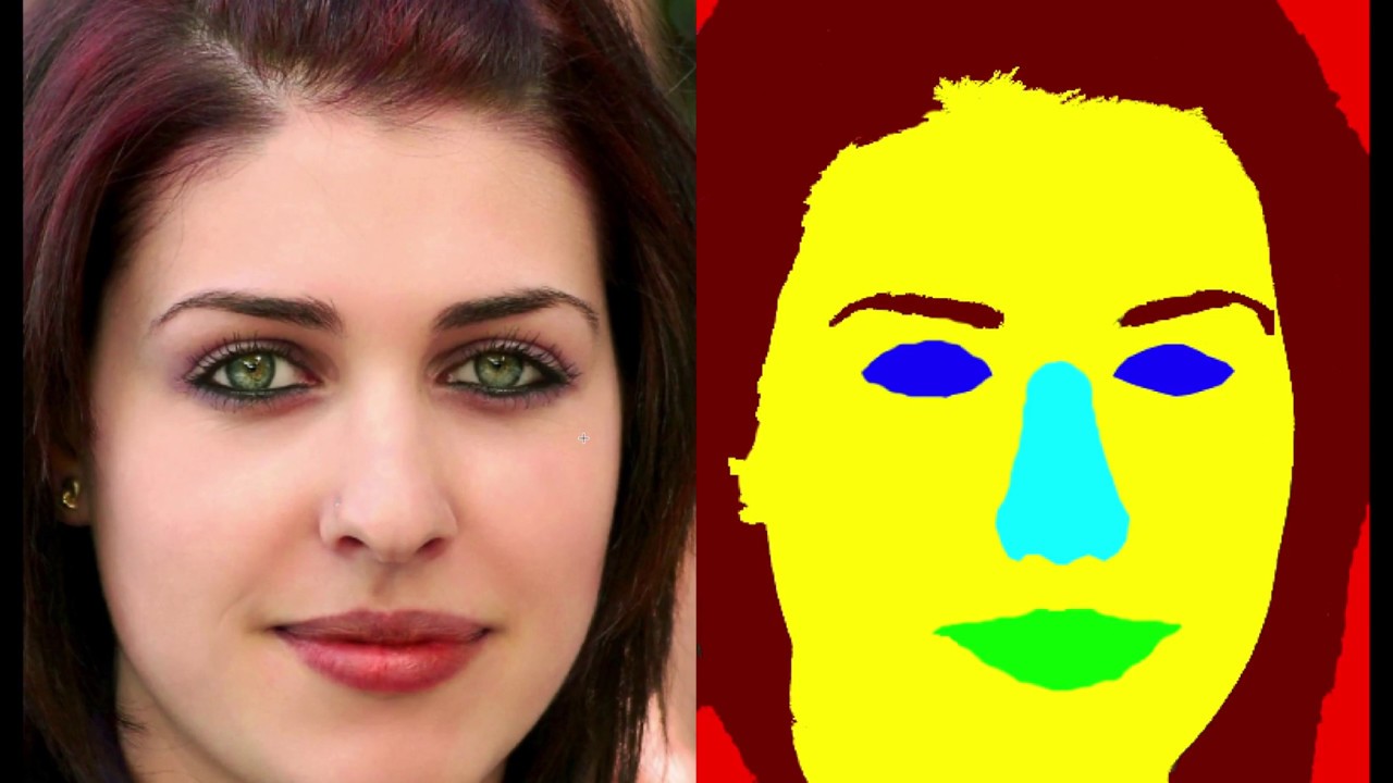
Source: https://github.com/massimomauro/FASSEG-repository/blob/master/papers/multiclass_face_segmentation_ICIP2015.pdf
Facial Segmentation is used for segmenting each part of the face into semantically similar regions – lips, eyes etc. This can be useful in many real-world applications. One very interesting application can be a virtual makeover.

2.3. Indoor Object Segmentation

Source: http://buildingparser.stanford.edu/dataset.html
Can you guess where this is used? In AR (Augmented Reality) and VR (Virtual Reality). AR applications can segment the entire indoor area to understand the position of chairs, tables, people, wall, and other similar objects, and thus, can place and manipulate virtual objects efficiently.
2.4. Geo Land Sensing

Source: https://www.sciencedirect.com/science/article/pii/S0924271616305305
Geo Land Sensing is a way of categorizing each pixel in satellite images into a category such that we can track the land cover of each area. If there is an area where heavy deforestation takes place, appropriate measures can be taken. There can be many more applications using semantic segmentation on satellite images.
Now that we know a few important applications of segmentation, let us see how to perform semantic segmentation using PyTorch and Torchvision. Here’s a video that will give you a glimpse of what’s to come.
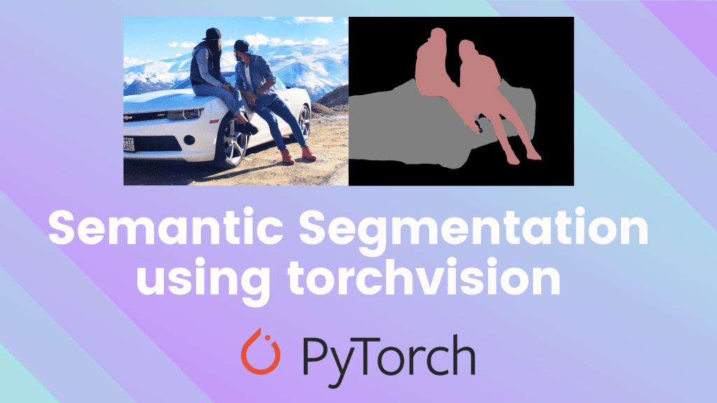
3. Semantic Segmentation using torchvision
We will look at two Deep Learning based models for Semantic Segmentation – Fully Convolutional Network ( FCN ) and DeepLab v3. These models have been trained on a subset of COCO Train 2017 dataset which corresponds to the PASCAL VOC dataset. There are a total of 20 categories supported by the models.
You can use the Colab Notebook to follow this tutorial and code.
3.1. Input and Output
Before we get started, let us understand the inputs and outputs of the models.
These models expect a 3-channel image (RGB) which is normalized with the Imagenet mean and standard deviation, i.e.mean = [0.485, 0.456, 0.406], std = [0.229, 0.224, 0.225]
So, the input dimension is [Ni x Ci x Hi x Wi]
where,
Ni-> the batch sizeCi-> the number of channels (which is 3)Hi-> the height of the imageWi-> the width of the image
And the output dimension of the model is [No x Co x Ho x Wo]
where,
No-> is the batch size (same asNi)Co-> is the number of classes that the dataset have!Ho-> the height of the image (which is the same asHiin almost all cases)Wo-> the width of the image (which is the same asWiin almost all cases)
NOTE: The output of torchvision models is an OrderedDict and not a torch.Tensor.During inference (.eval() mode ) the output, which is an OrderedDict has just one key – out. This out key holds the output and the corresponding values are in the shape of [No x Co x Ho x Wo].
Now, we are ready to play 🙂
3.2. FCN with Resnet-101 backbone
FCN – Fully Convolutional Networks are one of the first successful attempts of using Neural Networks for the task of Semantic Segmentation. We cover FCNs and few other models in great detail in our course on Deep Learning with PyTorch. For now, let us see how to use the model in Torchvision.
3.2.1. Load the model
Let’s load up the FCN!
from torchvision import models fcn = models.segmentation.fcn_resnet101(pretrained=True).eval()
And that’s it! Now, we have a pretrained model of FCN with a Resnet101 backbone. The pretrained=True flag will download the model if it is not already present in the cache. The .eval method will load it in the inference mode.
3.2.2. Load the Image
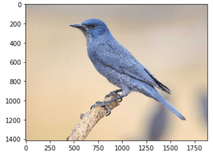
Next, let’s get an image! We download an image of a bird directly from a URL and save it. As you will see in the code, we use PIL to load the image.
from PIL import Image import matplotlib.pyplot as plt import torch !wget -nv https://static.independent.co.uk/s3fs-public/thumbnails/image/2018/04/10/19/pinyon-jay-bird.jpg -O bird.png img = Image.open(‘./bird.png’) plt.imshow(img); plt.show()
3.2.3. Pre-process the image
In order to prepare the image to be in the right format for inference using the model, we need to pre-process it and normalize it!
So, for the pre-processing steps, we carry out the following.
- Resize the image to
(256 x 256) - CenterCrop it to
(224 x 224) - Convert it to Tensor – all the values in the image will be scaled so they lie between
[0, 1]instead of the original,[0, 255]range. - Normalize it with the Imagenet specific values where
mean = [0.485, 0.456, 0.406], std = [0.229, 0.224, 0.225]
And lastly, we unsqueeze the image dimensions so that it becomes [1 x C x H x W] from [C x H x W]. This is required since we need a batch while passing it through the network.
# Apply the transformations needed import torchvision.transforms as T trf = T.Compose([T.Resize(256), T.CenterCrop(224), T.ToTensor(), T.Normalize(mean = [0.485, 0.456, 0.406], std = [0.229, 0.224, 0.225])]) inp = trf(img).unsqueeze(0)
Let’s see what the above code does.
Torchvision has many useful functions. One of them is Transforms which is used to pre-process images. T.Compose is a function that takes in a list in which each element is of transforms type. This returns an object through which we can pass batches of images and all the required transforms will be applied to all of the images.
Let’s take a look at the transforms applied on the images:
T.Resize(256): Resizes the image to size256 x 256T.CenterCrop(224): Center Crops the image to have a resulting size of224 x 224T.ToTensor(): Converts the image to typetorch.Tensorand scales the values to[0, 1]rangeT.Normalize(mean, std): Normalizes the image with the given mean and standard deviation.
3.2.4. Forward pass through the network
Now that we have an image which is preprocessed and ready, let’s pass it through the model and get the out key.
As mentioned earlier, the output of the model is an OrderedDict so we need to take the out key from it to obtain the output of the model.
# Pass the input through the net out = fcn(inp)[‘out’] print (out.shape)
torch.Size([1, 21, 224, 224])
So, out is the final output of the model. As we can see, its shape is [1 x 21 x H x W], as discussed earlier. Since, the model was trained on 21 classes, the output has 21 channels!
Now what we need to do is, make this 21 channelled output into a 2D image or a 1 channel image, where each pixel of that image corresponds to a class!
The 2D image (of shape [H x W]) will have each pixel corresponding to a class label. Note that each (x, y) pixel in this 2D image corresponds to a number between 0 - 20 representing a class.
The question now is how do we get there from the current image with dimensions [1 x 21 x H x W]?
Simple! We take a max index for each pixel position, which represents the class.
import numpy as np om = torch.argmax(out.squeeze(), dim=0).detach().cpu().numpy() print (om.shape)
(224, 224)
print (np.unique(om))
[0 3]
As we can observe after processing, we now have a 2D image where each pixel corresponds to a class. The last thing to do is to take this 2D image and convert it into a segmentation map where each class label is converted into an RGB color and thus helping in visualization.
3.2.5. Decode Output
We will use the following function to convert this 2D image to an RGB image where each label is mapped to its corresponding color.

# Define the helper function
def decode_segmap(image, nc=21):
  label_colors = np.array([(0, 0, 0),  # 0=background
               # 1=aeroplane, 2=bicycle, 3=bird, 4=boat, 5=bottle
               (128, 0, 0), (0, 128, 0), (128, 128, 0), (0, 0, 128), (128, 0, 128),
               # 6=bus, 7=car, 8=cat, 9=chair, 10=cow
               (0, 128, 128), (128, 128, 128), (64, 0, 0), (192, 0, 0), (64, 128, 0),
               # 11=dining table, 12=dog, 13=horse, 14=motorbike, 15=person
               (192, 128, 0), (64, 0, 128), (192, 0, 128), (64, 128, 128), (192, 128, 128),
               # 16=potted plant, 17=sheep, 18=sofa, 19=train, 20=tv/monitor
               (0, 64, 0), (128, 64, 0), (0, 192, 0), (128, 192, 0), (0, 64, 128)])
  r = np.zeros_like(image).astype(np.uint8)
  g = np.zeros_like(image).astype(np.uint8)
  b = np.zeros_like(image).astype(np.uint8)
  for l in range(0, nc):
    idx = image == l
    r[idx] = label_colors[l, 0]
    g[idx] = label_colors[l, 1]
    b[idx] = label_colors[l, 2]
  rgb = np.stack([r, g, b], axis=2)
  return rgb
Let’s see what we are doing inside this function!
First, the variable label_colors stores the colors for each of the classes according to the index. So, the color for the first class which is background is stored at the 0th index of the label_colors list. The second class, which is aeroplane, is stored at index 1 and so on.
Now, we have to create an RGB image from the 2D image we have. So, what we do is that we create empty 2D matrices for all the 3 channels.
So, r, g, and b are arrays which will form the RGB channels for the final image. Each of these arrays is of shape [H x W] (which is the same as the shape of the 2Dimage).
Now, we loop over each class color we stored in label_colors and we obtain the corresponding indexes in the image where that particular class label is present. Then for each channel, we put its corresponding color to those pixels where that class label is present.
Finally, we stack the 3 separate channels together to form a RGB image.
Now, let’s use this function to see the final segmented output!
rgb = decode_segmap(om)
plt.imshow(rgb); plt.show()
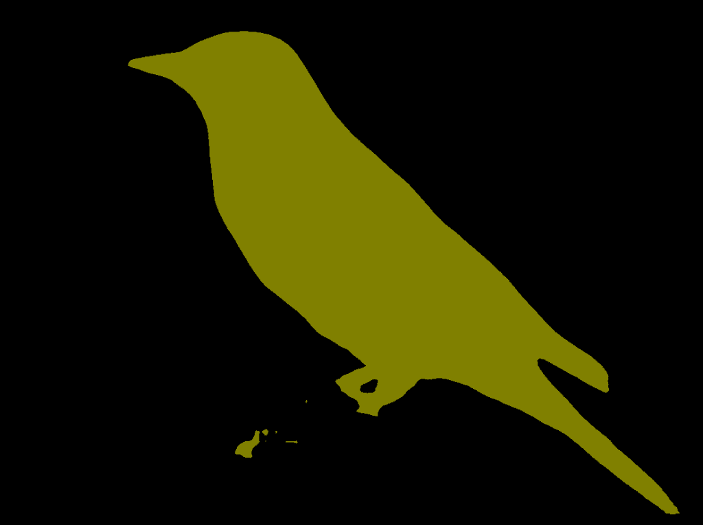
And there we go! We have segmented the output of the image.
That’s the bird!
Note: the image after segmentation is smaller than the original image as the image is resized and cropped in the preprocessing step.
3.2.6. Final Result
Next, let’s move all this into one single function and play around with a few more images!
def segment(net, path):
  img = Image.open(path)
  plt.imshow(img); plt.axis('off'); plt.show()
  # Comment the Resize and CenterCrop for better inference results
  trf = T.Compose([T.Resize(256),
                   T.CenterCrop(224),
                   T.ToTensor(),
                   T.Normalize(mean = [0.485, 0.456, 0.406],
                               std = [0.229, 0.224, 0.225])])
  inp = trf(img).unsqueeze(0)
  out = net(inp)['out']
  om = torch.argmax(out.squeeze(), dim=0).detach().cpu().numpy()
  rgb = decode_segmap(om)
  plt.imshow(rgb); plt.axis('off'); plt.show()
Let’s get a new image!
!wget -nv https://learnopencv.com/wp-content/uploads/2021/01/horse-segmentation.jpeg -O horse.png segment(fcn, './horse.png')
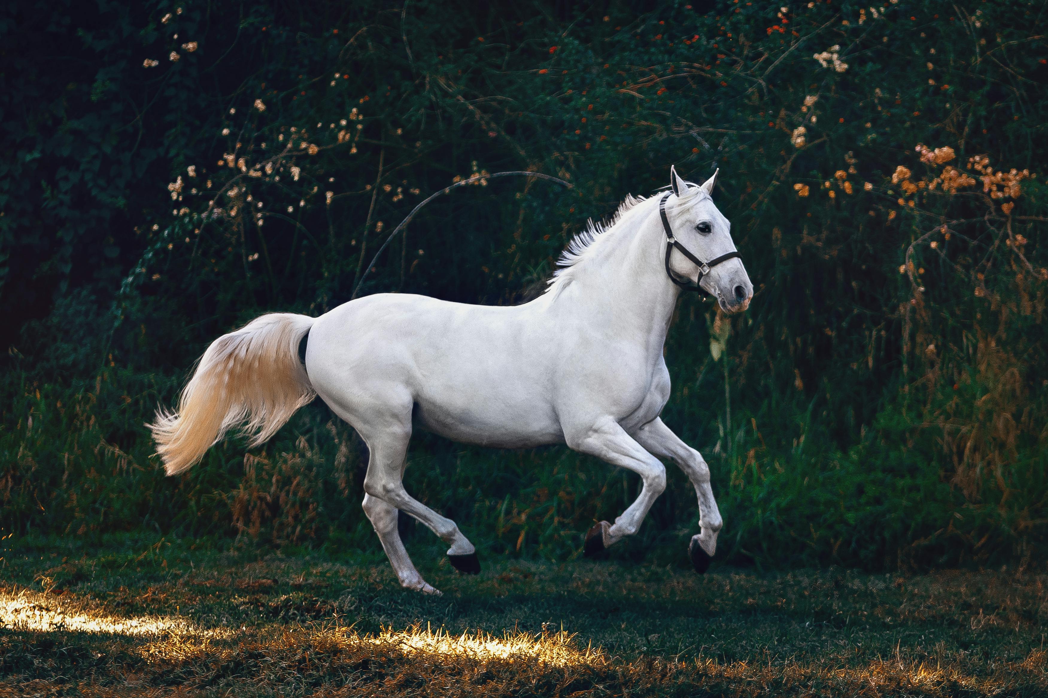
Wasn’t that interesting? Now let’s move on to one of the State-of-the-Art architectures in Semantic Segmentation – DeepLab.
3.3. Semantic Segmentation using DeepLab
DeepLab is a Semantic Segmentation Architecture that came out of Google Brain. Let’s see how we can use it.
dlab = models.segmentation.deeplabv3_resnet101(pretrained=1).eval()
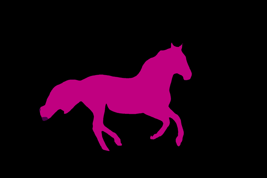
Let’s see how we can perform semantic segmentation on the same image using this model! We will use the same function we defined above.
segment(dlab, './horse.png')

So, there you go! You can see that, the DeepLab model has segmented the horse almost perfectly!
3.4. Multiple Objects
When we take a more complex image with multiple objects, then we can start to see some differences in the results obtained using both the models.
Let’s try that out!
!wget -nv "https://learnopencv.com/wp-content/uploads/2021/01/person-segmentation.jpeg" -O dog-park.png
img = Image.open('./dog-park.png')
plt.imshow(img); plt.show()
print ('Segmenatation Image on FCN')
segment(fcn, path='./dog-park.png', show_orig=False)
print ('Segmenatation Image on DeepLabv3')
segment(dlab, path='./dog-park.png', show_orig=False)
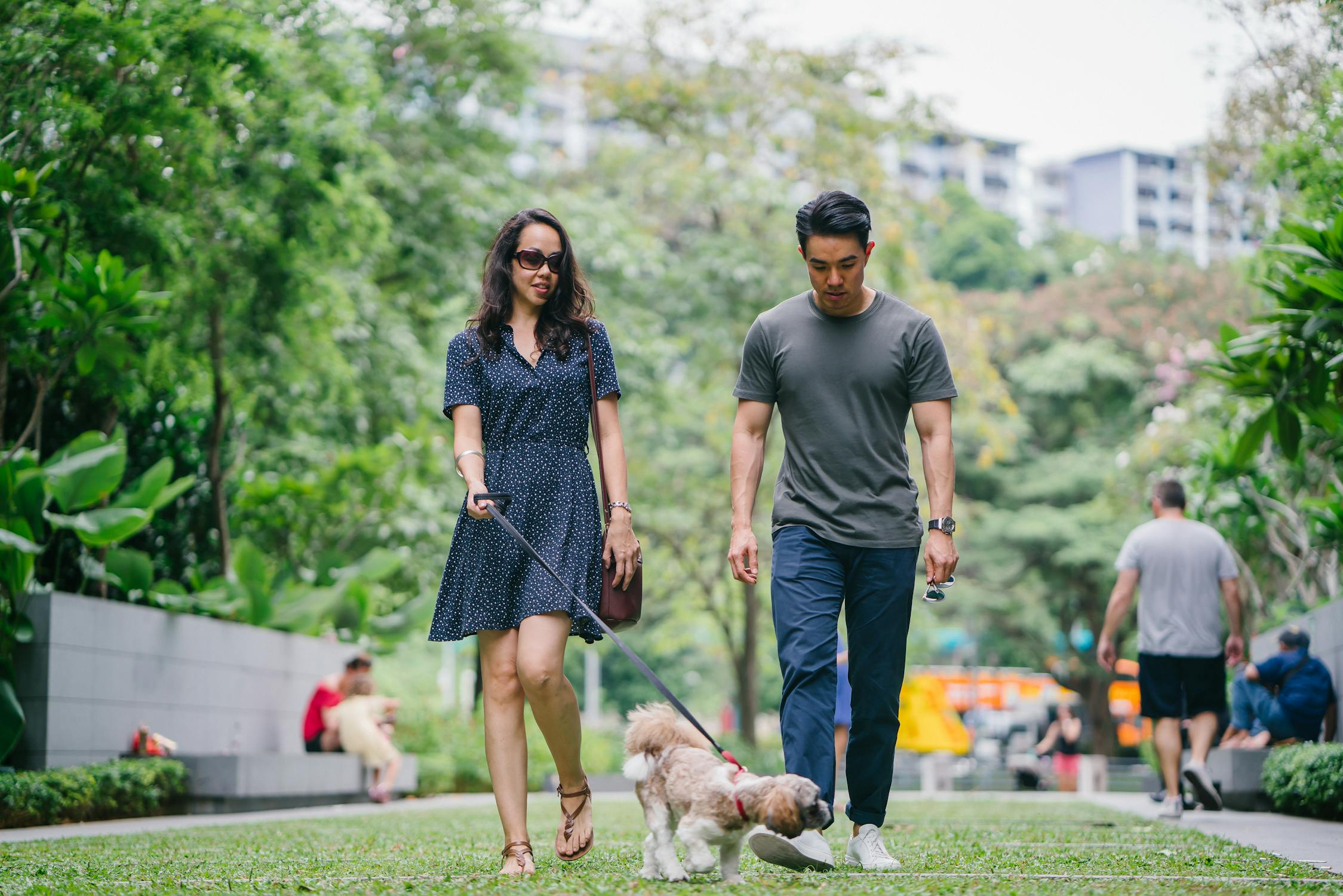
Source: Pexels
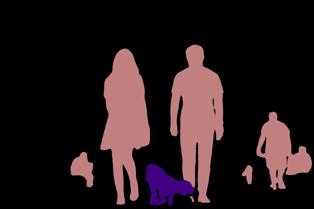
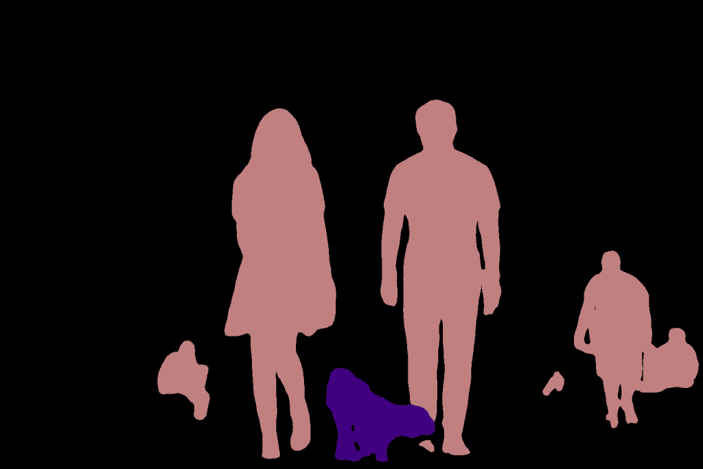
As you can see both the models perform quite well! However, there are cases where the model fails miserably.
4. Comparison
Till now we have seen how the code works and how the outputs look qualitatively. In this section, we will discuss the quantitative aspects of the models. We will also compare the two models with each other on the basis of the following 3 metrics.
- Inference time on CPU and GPU
- Size of the model.
- GPU memory used while inference.
4.1. Inference Time
We have used Google Colab to run the code and get to these numbers. You can check out the code for the same in the shared notebooks.
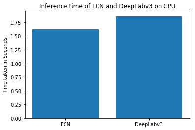
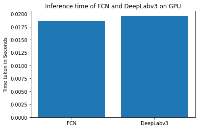
We can see that DeepLab model is slightly slower than FCN.
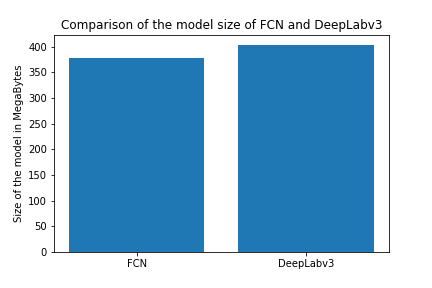
4.2. Model Size
Model size is the size of the weights file for the model. DeepLab is a slightly bigger model than FCN.
4.3. GPU Memory requirements
We have used a NVIDIA GTX 1080 Ti GPU for this and found that both models take around 1.2GB for a 224×224 sized image.
In our next posts, we will discuss other computer vision problems using PyTorch and Torchvision. Stay tuned!
Check out these posts:
PyTorch Tutorial for Beginners
PyTorch for Beginners: Image Classification using Pre-trained models


