Transfer Learning For Pytorch Image Classification

Transfer Learning has revolutionized the way we approach image classification in PyTorch. Recently PyTorch has gained a lot of popularity because of its ease of usage and learning. Andrej Karpathy, Senior Director of AI at Tesla, said the following in his tweet.

Jokes apart, PyTorch is very transparent and can help researchers and data scientists achieve high productivity and reliable results.

This article is part of the following series:

In this post, we discuss image classification in PyTorch. We will use a subset of the CalTech256 dataset to classify images of 10 animals. We will go over the steps of dataset preparation, data augmentation and then the steps to build the classifier. We use transfer learning to use the low level image features like edges, textures etc. These are learnt by a pretrained model, ResNet50, and then train our classifier to learn the higher level details in our dataset images like eyes, legs etc. ResNet50 has already been trained on ImageNet with millions of images. In another article on blog we disuss Transfer Learning for Medical Images.

Do not worry about functions and code. The post has code snippets to make it easy to study and understand. Also, the complete code has been made available over a python notebook (subscribe and download for free). Before we dive into the article, here’s a video on Pytorch image classification to motivate you further. Just like this video shows, you could build your own “Zoo classifier”!

While we have tried to make the post self-sufficient, we still encourage the readers to get familiarized to the Basics of Pytorch before proceeding further.

Dataset Preparation

The CalTech256 dataset has 30,607 images categorized into 256 different labeled classes along with another ‘clutter’ class.

Training the whole dataset will take hours. So we will work on a subset of the dataset containing 10 animals – bear, chimp, giraffe, gorilla, llama, ostrich, porcupine, skunk, triceratops, and zebra. That way we can experiment faster. The code can then be used to train the whole dataset too.

The number of images in these folders varies from 81(for a skunk) to 212(for a gorilla). We use the first 60 images in each of these categories for training. The next 10 images are for validation, and the rest are for testing in our experiments below.

So finally, we have 600 training images, 100 validation images, 409 test images, and 10 classes of animals.

If you want to replicate the experiments, please follow the steps below

1. Download the CalTech256 dataset
2. Create three directories with names train, valid and test.
3. Create 10 sub-directories each inside the train and the test directories. The sub-directories should be named bear, chimp, giraffe, gorilla, llama, ostrich, porcupine, skunk, triceratops and zebra.
4. Move the first 60 images for bear in the Caltech256 dataset to the directory train/bear. Repeat this step for every animal.
5. Move the next 10 images for bear in the Caltech256 dataset to the directory valid/bear. Repeat this step for every animal.
6. Copy the remaining images for bear (i.e. the ones not included in a train or valid folders) to the directory test/bear. Repeat this step for every animal.

Data Augmentation

The images in the available training set can be modified several ways to incorporate more variations in the training process. This way, the trained model gets more generalized and performs well on different test data. Also, the input data can come in a variety of sizes. They need to be normalized to a fixed size and format before batches of data are used together for training.

First, each of the input images is passed through many transformations. We try to insert some variations by introducing some randomness into the transformations. In each epoch, a single set of transformations are applied to each image. When we train for multiple epochs, the models see more variations of the input images with a new randomized variation of the transformation in each epoch. This results in data augmentation, and the model then tries to generalize more.

Below we see an example of the transformed versions of a Triceratops image.

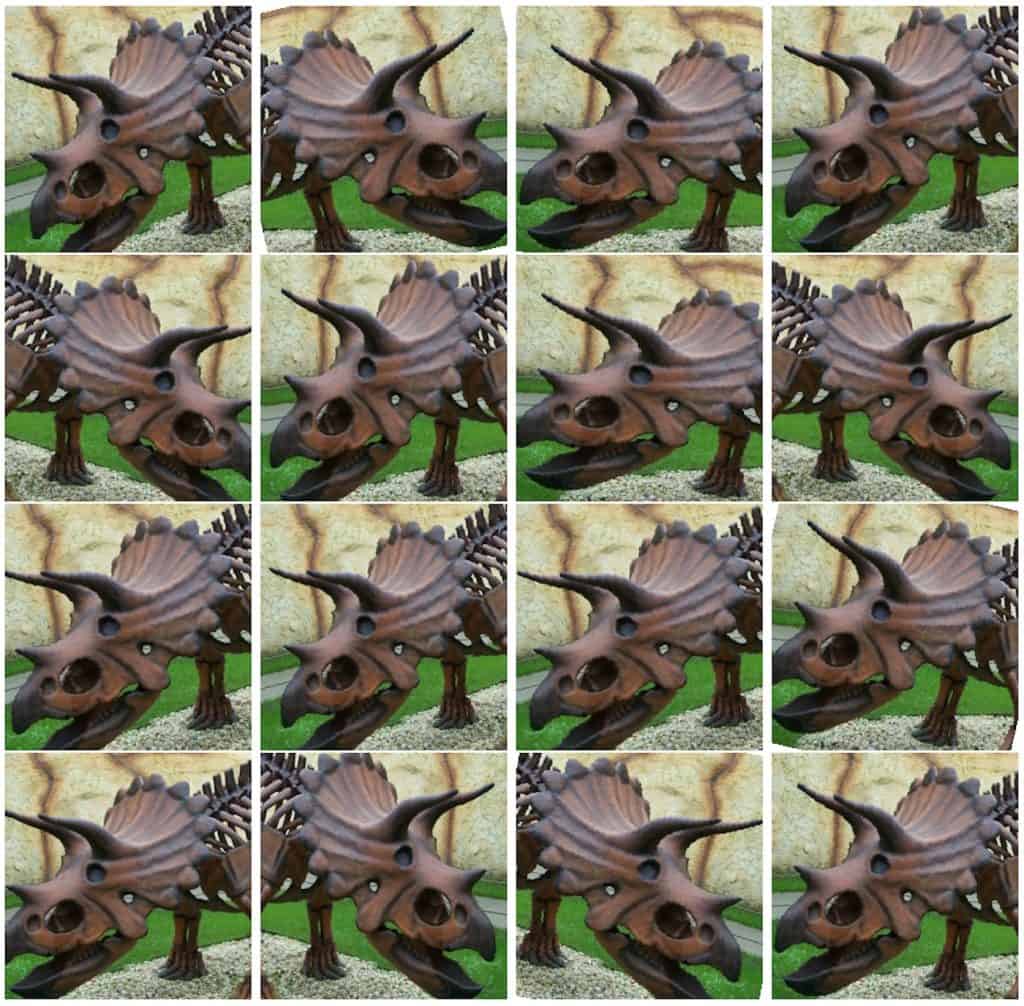
Let us go over the transformations we used for our data augmentation.

The transform RandomResizedCrop crops the input image by a random size(within a scale range of 0.8 to 1.0 of the original size and a random aspect ratio in the default range of 0.75 to 1.33 ). The cropped image is then resized to 256×256.

RandomRotation rotates the image by a random angle in the range of -15 to 15 degrees.

RandomHorizontalFlip randomly flips the image horizontally with a default probability of 50%.

CenterCrop crops a 224×224 image from the center.

ToTensor converts the PIL Image with values in the range of 0-255 to a floating point Tensor and normalizes them to a range of 0-1, by dividing it by 255.

Normalize takes in a 3 channel Tensor and normalizes each channel by the input mean and standard deviation for that channel. Mean and standard deviation vectors are input as 3 element vectors. Each channel in the tensor is normalized as T = (T – mean)/(standard deviation)

All the above transformations are chained together using Compose.

Click here to download the source code to this post

# Applying Transforms to the Data
image_transforms = { 
    'train': transforms.Compose([
        transforms.RandomResizedCrop(size=256, scale=(0.8, 1.0)),
        transforms.RandomRotation(degrees=15),
        transforms.RandomHorizontalFlip(),
        transforms.CenterCrop(size=224),
        transforms.ToTensor(),
        transforms.Normalize([0.485, 0.456, 0.406],
                             [0.229, 0.224, 0.225])
    ]),
    'valid': transforms.Compose([
        transforms.Resize(size=256),
        transforms.CenterCrop(size=224),
        transforms.ToTensor(),
        transforms.Normalize([0.485, 0.456, 0.406],
                             [0.229, 0.224, 0.225])
    ]),
    'test': transforms.Compose([
        transforms.Resize(size=256),
        transforms.CenterCrop(size=224),
        transforms.ToTensor(),
        transforms.Normalize([0.485, 0.456, 0.406],
                             [0.229, 0.224, 0.225])
    ])
}

Note that for the validation and test data, we do not do the RandomResizedCrop, RandomRotation and RandomHorizontalFlip transformations. Instead, we resize the validation images to 256×256 and crop out the center 224×224 to be able to use them with the pretrained model. Finally, the image is transformed into a tensor and normalized by the mean and standard deviation of all the images in ImageNet.

Data Loading

Next, let us see how to use the above-defined transformations and load the data to be used for training.

# Load the Data
# Set train and valid directory paths
train_directory = 'train'
valid_directory = 'test'
# Batch size
bs = 32
# Number of classes
num_classes = 10
# Load Data from folders
data = {
    'train': datasets.ImageFolder(root=train_directory, transform=image_transforms['train']),
    'valid': datasets.ImageFolder(root=valid_directory, transform=image_transforms['valid']),
    'test': datasets.ImageFolder(root=test_directory, transform=image_transforms['test'])
}
# Size of Data, to be used for calculating Average Loss and Accuracy
train_data_size = len(data['train'])
valid_data_size = len(data['valid'])
test_data_size = len(data['test'])
# Create iterators for the Data loaded using DataLoader module
train_data = DataLoader(data['train'], batch_size=bs, shuffle=True)
valid_data = DataLoader(data['valid'], batch_size=bs, shuffle=True)
test_data = DataLoader(data['test'], batch_size=bs, shuffle=True)
# Print the train, validation and test set data sizes
train_data_size, valid_data_size, test_data_size

We first set the train and validation data directories and the batch size. Then we load them using DataLoader. Note that the image transformations we discussed earlier are applied to the data while loading them using the DataLoader. The order of the data is also shuffled. The torchvision.transforms package and the DataLoader are important PyTorch features that make the data augmentation and loading processes very easy.

Transfer Learning

It is very hard and time consuming to collect images belonging to a domain of interest and train a classifier from scratch. So, we use a pre-trained model as our base and change the last few layers to classify images according to our desirable classes. This helps us get good results even with a small dataset since the basic image features have already been learned in the pre-trained model from a much larger dataset like ImageNet.

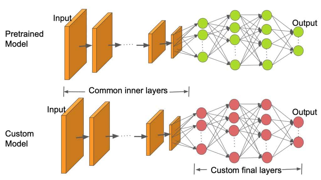
As we can see in the above image, the inner layers are kept the same as the pretrained model and only the final layers are changed to fit our number of classes. In this work, we use the pre-trained ResNet50 model.

# Load pretrained ResNet50 Model
resnet50 = models.resnet50(pretrained=True)

Canziani et al. list many pretrained models that are used for various practical applications, analyzing the accuracy obtained and the inference time needed for each model. ResNet50 is one model with a good tradeoff between accuracy and inference time. When a model is loaded in PyTorch, all its parameters have their ‘requires_grad’ field set to true by default. This means each and every change to the parameter values will be stored to be used in the backpropagation graph used for training. This increases memory requirements. Since most of the parameters in our pre-trained model are already trained, we reset the requires_grad field to false.

# Freeze model parameters
for param in resnet50.parameters():
    param.requires_grad = False

Next, we replace the final layer of the ResNet50 model by a small set of Sequential layers. The inputs to the last fully connected layer of ResNet50 is fed to a Linear layer. It has 256 outputs, which are then fed into ReLU and Dropout layers. It is then followed by a 256×10 Linear Layer which has 10 outputs corresponding to the 10 classes in our CalTech subset.

# Change the final layer of ResNet50 Model for Transfer Learning
fc_inputs = resnet50.fc.in_features
resnet50.fc = nn.Sequential(
    nn.Linear(fc_inputs, 256),
    nn.ReLU(),
    nn.Dropout(0.4),
    nn.Linear(256, 10), 
    nn.LogSoftmax(dim=1) # For using NLLLoss()
)

Since we will be training on a GPU, we get the model ready for GPU.

# Convert model to be used on GPU
resnet50 = resnet50.to('cuda:0')

Next, we define the loss function and the optimizer to be used for training. PyTorch provides a variety of loss functions. We use the Negative Loss Likelihood function as it is useful for classifying multiple classes. PyTorch also supports multiple optimizers. We use the Adam optimizer. Adam is one of the most popular optimizers because it can adapt the learning rate for each parameter individually.

# Define Optimizer and Loss Function
loss_func = nn.NLLLoss()
optimizer = optim.Adam(resnet50.parameters())

Training

The complete training code is in the python notebook, but we will discuss the main concept here. Training is carried out for a fixed set of epochs, processing each image once in a single epoch. The training data loader loads data in batches. In our case, we have given a batch size of 32. This means each batch can have a maximum of 32 images.

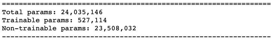
For each batch, input images are passed through the model, a.k.a forward pass, to get the outputs. Then the provided loss_criterion or cost function is used to compute the loss using the ground truth and the computed outputs. The gradients of the loss with respect to the trainable parameters are computed using the backward function. Note that with transfer learning, we need to compute gradients only for a small set of parameters that belong to the few newly added layers toward the end of the model. A summary function call to the model can reveal the actual number of parameters and the number of trainable parameters. The advantage we have in this approach is we now need to train only around a tenth of the total number of model parameters.

Gradient computation is done using the autograd and backpropagation, differentiating in the graph using the chain rule. PyTorch accumulates all the gradients in the backward pass. So it is essential to zero them out at the beginning of the training loop. This is achieved using the optimizer’s zero_grad function. Finally, after the gradients are computed in the backward pass, the parameters are updated using the optimizer’s step function.

Total loss and accuracy is computed for the whole batch, which is then averaged over all the batches to get the loss and accuracy values for the whole epoch.

for epoch in range(epochs):
        epoch_start = time.time()
        print("Epoch: {}/{}".format(epoch+1, epochs))
        # Set to training mode
        model.train()
        # Loss and Accuracy within the epoch
        train_loss = 0.0
        train_acc = 0.0
        valid_loss = 0.0
        valid_acc = 0.0
        for i, (inputs, labels) in enumerate(train_data_loader):
            inputs = inputs.to(device)
            labels = labels.to(device)
            # Clean existing gradients
            optimizer.zero_grad()
            # Forward pass - compute outputs on input data using the model
            outputs = model(inputs)
            # Compute loss
            loss = loss_criterion(outputs, labels)
            # Backpropagate the gradients
            loss.backward()
            # Update the parameters
            optimizer.step()
            # Compute the total loss for the batch and add it to train_loss
            train_loss += loss.item() * inputs.size(0)
            # Compute the accuracy
            ret, predictions = torch.max(outputs.data, 1)
            correct_counts = predictions.eq(labels.data.view_as(predictions))
            # Convert correct_counts to float and then compute the mean
            acc = torch.mean(correct_counts.type(torch.FloatTensor))
            # Compute total accuracy in the whole batch and add to train_acc
            train_acc += acc.item() * inputs.size(0)
            print("Batch number: {:03d}, Training: Loss: {:.4f}, Accuracy: {:.4f}".format(i, loss.item(), acc.item()))

Validation

As training is carried out for more epochs, the model tends to overfit the data leading to its poor performance on new test data. Maintaining a separate validation set is important, so we can stop the training at the right point and prevent overfitting. Validation is carried out in each epoch immediately after the training loop. Since we do not need any gradient computation in the validation process, it is done within a torch.no_grad() block.

For each validation batch, the inputs and labels are transferred to the GPU ( if cuda is available, else they are transferred to the CPU). The inputs go through the forward pass, followed by the loss and accuracy computations for the batch and at the end of the loop, for the whole epoch.

# Validation - No gradient tracking needed
        with torch.no_grad():
            # Set to evaluation mode
            model.eval()
            # Validation loop
            for j, (inputs, labels) in enumerate(valid_data_loader):
                inputs = inputs.to(device)
                labels = labels.to(device)
                # Forward pass - compute outputs on input data using the model
                outputs = model(inputs)
                # Compute loss
                loss = loss_criterion(outputs, labels)
                # Compute the total loss for the batch and add it to valid_loss
                valid_loss += loss.item() * inputs.size(0)
                # Calculate validation accuracy
                ret, predictions = torch.max(outputs.data, 1)
                correct_counts = predictions.eq(labels.data.view_as(predictions))
                # Convert correct_counts to float and then compute the mean
                acc = torch.mean(correct_counts.type(torch.FloatTensor))
                # Compute total accuracy in the whole batch and add to valid_acc
                valid_acc += acc.item() * inputs.size(0)
                print("Validation Batch number: {:03d}, Validation: Loss: {:.4f}, Accuracy: {:.4f}".format(j, loss.item(), acc.item()))
        # Find average training loss and training accuracy
        avg_train_loss = train_loss/train_data_size 
        avg_train_acc = train_acc/float(train_data_size)
        # Find average training loss and training accuracy
        avg_valid_loss = valid_loss/valid_data_size 
        avg_valid_acc = valid_acc/float(valid_data_size)
        history.append([avg_train_loss, avg_valid_loss, avg_train_acc, avg_valid_acc])
        epoch_end = time.time()
        print("Epoch : {:03d}, Training: Loss: {:.4f}, Accuracy: {:.4f}%, nttValidation : Loss : {:.4f}, Accuracy: {:.4f}%, Time: {:.4f}s".format(epoch, avg_train_loss, avg_train_acc*100, avg_valid_loss, avg_valid_acc*100, epoch_end-epoch_start))

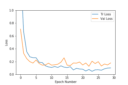
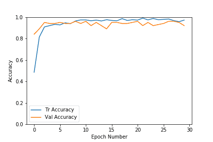
As we can see in the above plots, both the validation and training losses settle down pretty quickly for this dataset. The accuracy also increases up to the range of 0.9 very fast. As the number of epochs increases, the training loss decreases further, leading to overfitting, but the validation results do not improve much. So we chose the model from the epoch with higher accuracy and a lower loss. It is better if we stop early to prevent overfitting the training data. In our case, we chose epoch#8, which had a validation accuracy of 96%.

The early stopping process can also be automated. We can stop once the loss is below a threshold and if the validation accuracy does not improve for a given set of epochs.

Inference

Once we have the model, we can do inferences on individual test images or on the whole test dataset to obtain the test accuracy. The test set accuracy computation is similar to the validation code, except it is carried out on the test dataset. We have included the function computeTestSetAccuracy in the Python notebook for the same. Let us discuss below how to find the output class for a given test image.

An input image first undergoes all the transformations used for validation/test data. The resulting tensor is then converted to a 4-dimensional one and passed through the model, which outputs the log probabilities for different classes. An exponential of the model outputs provides us with the class probabilities. Then we choose the class with the highest probability as our output class.

Choose the class with the highest probability as our output class.

def predict(model, test_image_name):
    transform = image_transforms['test']
    test_image = Image.open(test_image_name)
    plt.imshow(test_image)
    test_image_tensor = transform(test_image)
    if torch.cuda.is_available():
        test_image_tensor = test_image_tensor.view(1, 3, 224, 224).cuda()
    else:
        test_image_tensor = test_image_tensor.view(1, 3, 224, 224)
    with torch.no_grad():
        model.eval()
        # Model outputs log probabilities
        out = model(test_image_tensor)
        ps = torch.exp(out)
        topk, topclass = ps.topk(1, dim=1)
        print("Output class :  ", idx_to_class[topclass.cpu().numpy()[0][0]])

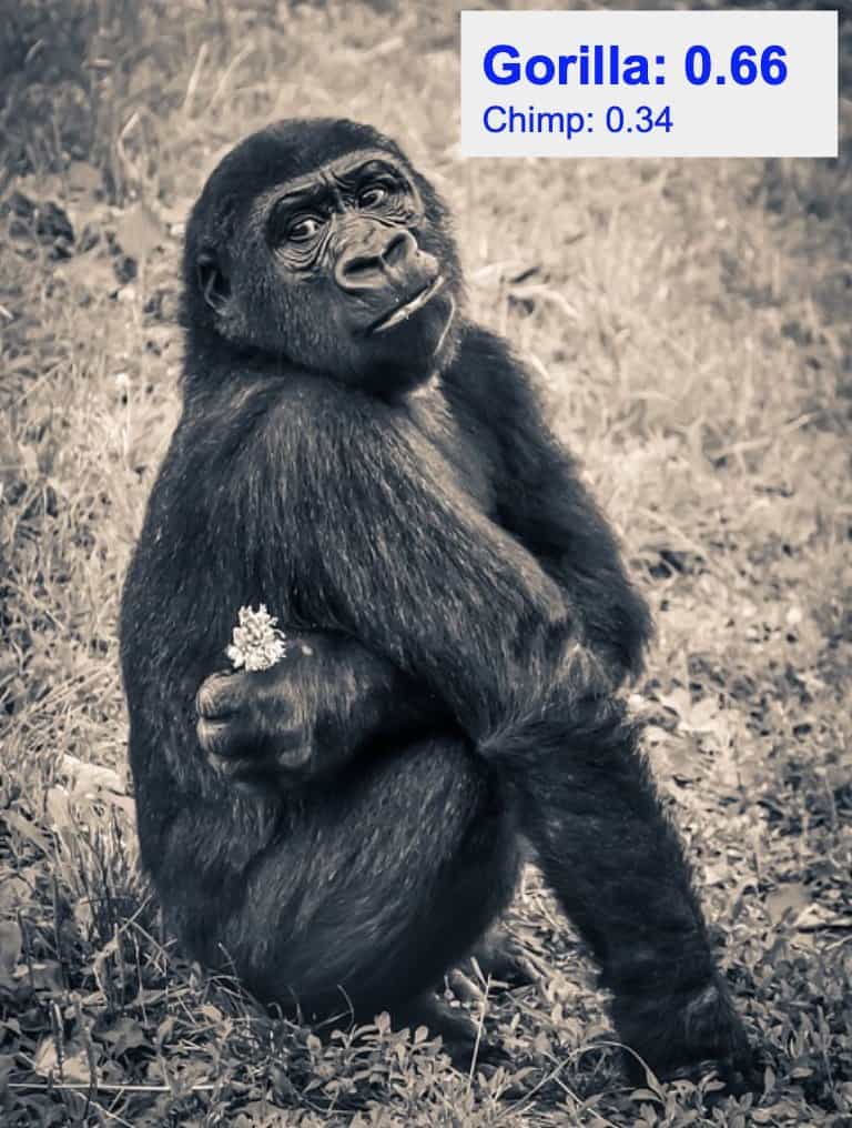
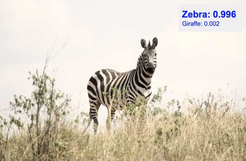
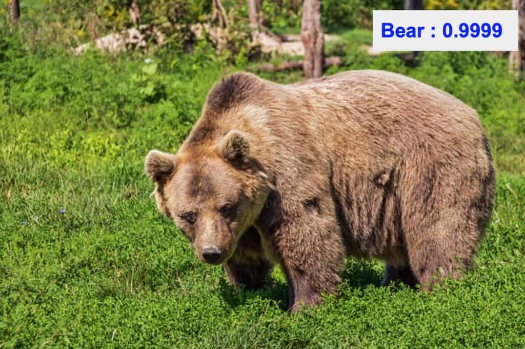
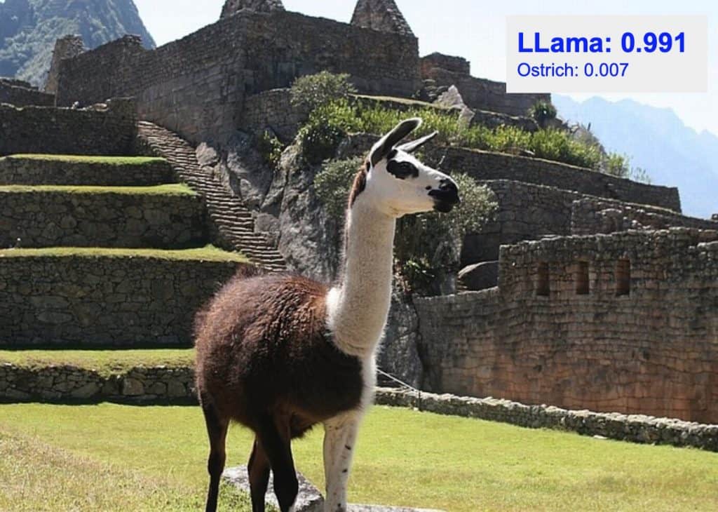
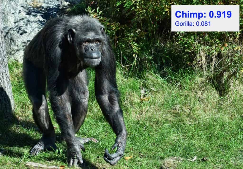
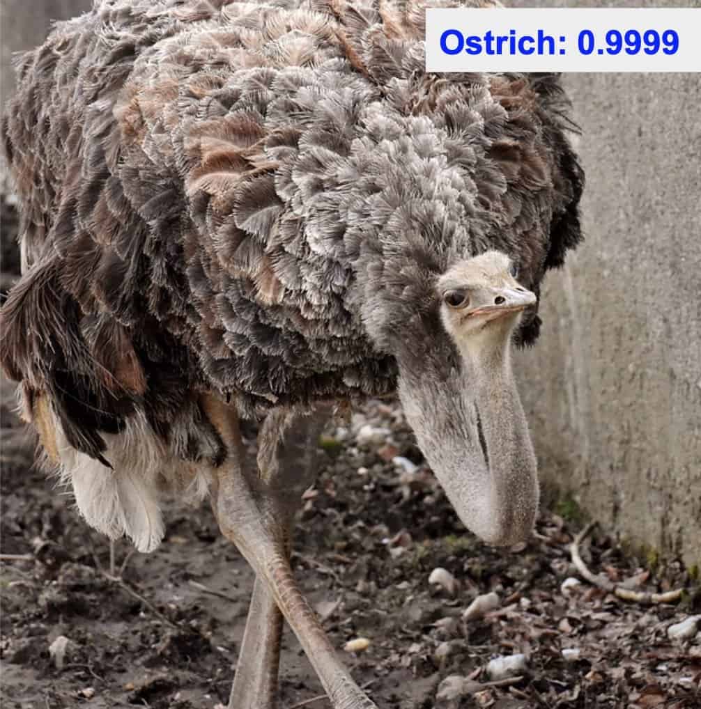
An accuracy of 92.4% was achieved on a test set with 409 images.

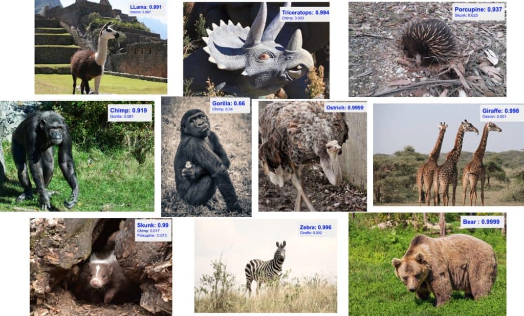
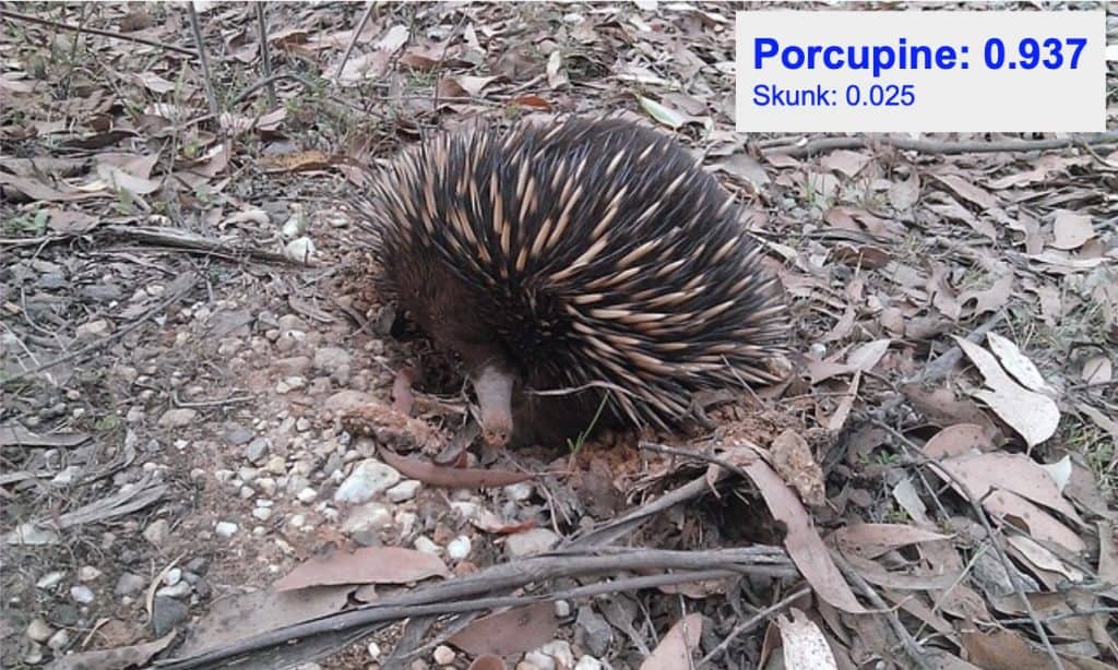
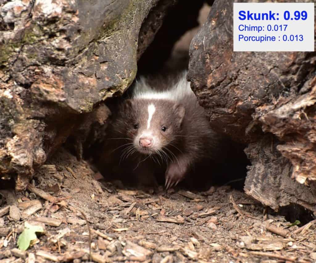
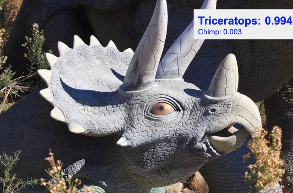
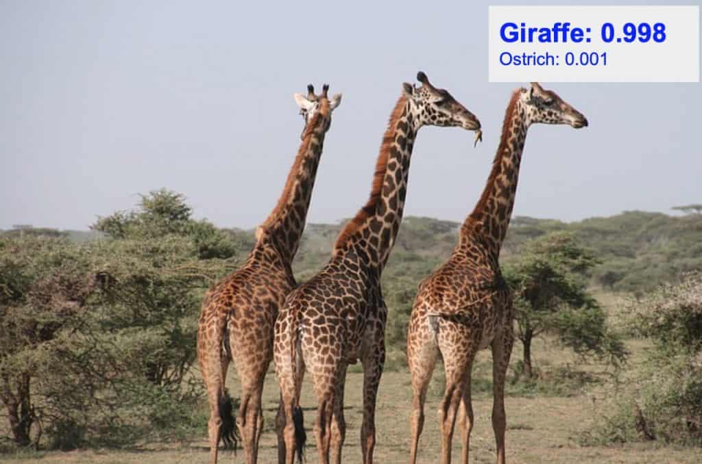
Below are some of the classification results on new test data that were not used in training or validation. The top predicted classes for the images with their probability scores are overlaid on the top right. As we see below, the class predicted with the highest probability is often the correct one. Also, note that the class with the second highest probability is often the closest animal in appearance to the actual class amongst all the remaining 9 classes.

We just saw how to use a pretrained model trained for 1000 classes of ImageNet. It very effectively classified images belonging to the 10 different classes of our interest.

We showed the classification results on a small dataset. In a future post, we will apply the same transfer learning approach on harder datasets solving harder real-life problems. Stay tuned!

Acknowledgement

I would like to thank our intern Kushashwa Ravi Shrimali for writing the code for this post.

Also check out our series on Getting Started With Pytorch.

References

• Griffin, Gregory and Holub, Alex and Perona, Pietro (2007) Caltech-256 Object Category Dataset.
• Pixabay Images used in the blog post: [1], [2], [3], [4], [5], [6], [7], [8], [9], [10], [11]